██████╗ ██████╗  ██████╗ ██████╗  ██████╗ ██╗   ██╗████████╗
██╔══██╗██╔══██╗██╔═══██╗██╔══██╗██╔═══██╗██║   ██║╚══██╔══╝
██║  ██║██████╔╝██║   ██║██████╔╝██║   ██║██║   ██║   ██║
██║  ██║██╔══██╗██║   ██║██╔═══╝ ██║   ██║██║   ██║   ██║
██████╔╝██║  ██║╚██████╔╝██║     ╚██████╔╝╚██████╔╝   ██║
╚═════╝ ╚═╝  ╚═╝ ╚═════╝ ╚═╝      ╚═════╝  ╚═════╝    ╚═╝
In the noisy classroom of a neural network, Dropout plays the role of the unpredictable professor — one who randomly sends half the students out for coffee breaks, mid-lecture. The goal? To make sure no single student becomes too smart for their own good. Dropout doesn’t just reduce overfitting — it teaches resilience. By deliberately "dropping out" neurons during training, we force the network to stop relying on any single path to the answer. Think of it as intellectual redundancy, hardwired.
Imagine a neural network as a grand orchestra, each neuron a musician playing their part. Dropout is like the conductor who randomly silences half the musicians during practice. The remaining musicians must adapt, improvise, and still create beautiful music. This way, when the full orchestra plays together, it’s more robust and harmonious.
Motivation and Early Works
But why did people want dropout? How did they even think of it? What was their motivation?Let us remember that deep Neural Networks can learn really complicated relationships between their inputs and outputs. This makes them a superpower as they can learn... almost every relation.
But there is a catch. What if you have less training data ? Will you have a close approximation of the hypothesis function ? (hypothesis function is the actual function that causes the data distribution; NN tries to be as close to it as possible..)
Well the answer is NO. But why? It is because the model learns to recognize sampling noise as a part of distribution data and begins to overfit.
But aren't there so many methods to prevent overfitting ?
There are several such ways, like:
- Stopping training as soon as validation accuracy begins to decrease.
- Using L1 and L2 regularization.
- Soft weight sharing.
Then why not use regularization methods above ?
This is due to issue of co-adaptation. In order to get the desired output, neurons can cheat by learning mutually dependent patterns. For example - Neuron A only fires if Neuron B does too. Together they encode something complex, but separately they're useless.
This means that the model memorizes shortcuts, and does not generalize.
| Technique | What it does | What it fails to address |
|---|---|---|
| L2 (Ridge) | Penalizes large weights
(∑ wi2) to reduce overfitting |
Doesn't prevent neurons from "collaborating" too tightly (co-adaptation) |
| L1 (Lasso) | Encourages sparsity by driving some weights to zero | Still allows hidden units to rely on each other too much |
| Both | Regularize individual weights | Don't regularize dependencies between neurons |
Okay, so we need better ways than just regularization; enter Bayesian Neural Nets.
A Bayesian Neural Network (BNN) is a neural network that treats weights as probability distributions rather than fixed values. It brings the principles of Bayesian inference into deep learning, allowing the model to estimate uncertainty in predictions.
The only problem that comes with it is its computational overhead. It requires far more forward passes, as well as variational inferences for approximating the posterior. Basically, things ain't that simple anymore.
Due to this, dropout stands as an effective way of regularization without co-adaptation.
Dropout simulates a given Neural net as an ensemble of different Neural nets with variable connections. This enables it to have more robust and generalizable neurons.
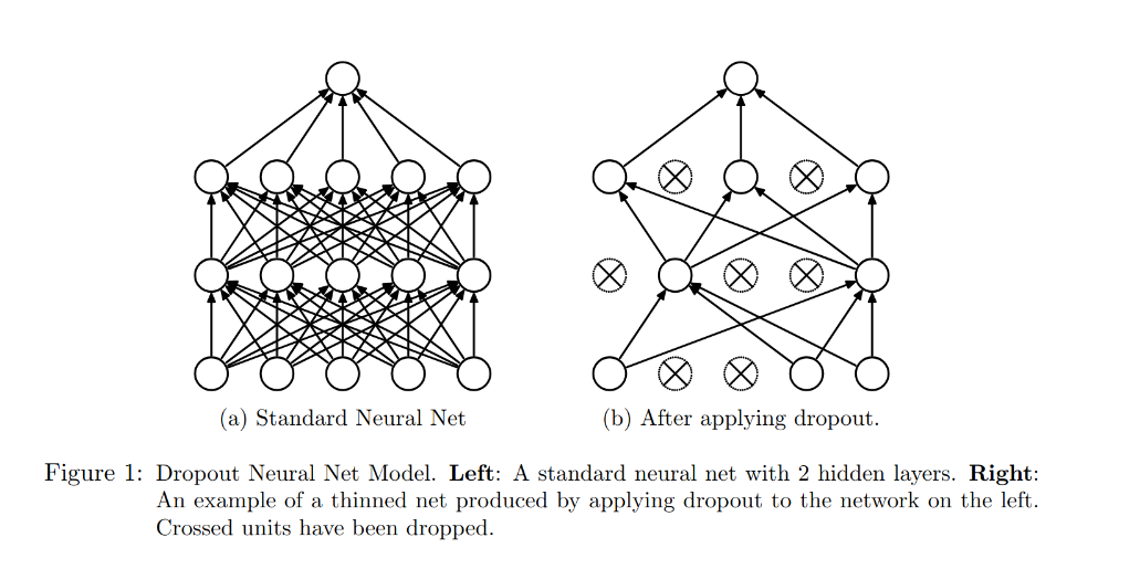
Dropout prevents overfitting and provides a way of approximately combining exponentially many different neural network architectures efficiently. The term “dropout” refers to dropping out units (hidden and visible) in a neural network. By dropping a unit out, we mean temporarily removing it from the network, along with all its incoming and outgoing connections. The choice of which one to remove is random.
Model Description
This section describes the dropout neural network model. Consider a neural network with \( L \) hidden layers. Let \( l \in \{1, \dots, L\} \) index the hidden layers of the network. Let \( \mathbf{z}^{(l)} \) denote the vector of inputs into layer \( l \), \( \mathbf{y}^{(l)} \) denote the vector of outputs from layer \( l \) (\( \mathbf{y}^{(0)} = \mathbf{x} \) is the input). \( \mathbf{W}^{(l)} \) and \( \mathbf{b}^{(l)} \) are the weights and biases at layer \( l \).
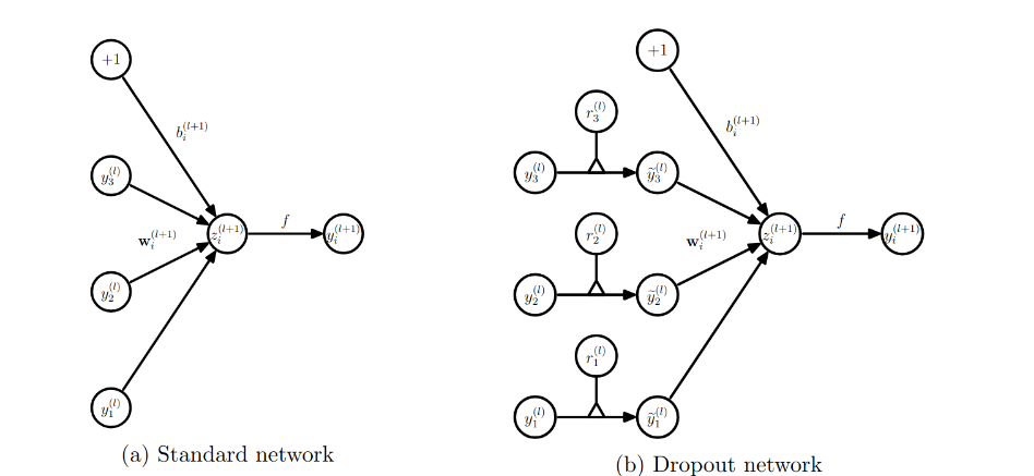
The feed-forward operation of a standard neural network can be described as (for \( l \in \{0, \dots, L-1\} \) and any hidden unit \( i \)):
\[ \begin{aligned} z^{(l+1)}_i &= \mathbf{w}^{(l+1)}_i \cdot \mathbf{y}^{(l)} + b^{(l+1)}_i \\ y^{(l+1)}_i &= f(z^{(l+1)}_i) \end{aligned} \]where \( f \) is any activation function, for example, \( f(x) = \frac{1}{1 + \exp(-x)} \).
With dropout, the feed-forward operation becomes:
\[ \begin{aligned} r^{(l)}_j &\sim \text{Bernoulli}(p) \\ \tilde{\mathbf{y}}^{(l)} &= \mathbf{r}^{(l)} * \mathbf{y}^{(l)} \\ z^{(l+1)}_i &= \mathbf{w}^{(l+1)}_i \cdot \tilde{\mathbf{y}}^{(l)} + b^{(l+1)}_i \\ y^{(l+1)}_i &= f(z^{(l+1)}_i) \end{aligned} \]Here, \( * \) denotes an element-wise (Hadamard) product. For any layer \( l \), \( \mathbf{r}^{(l)} \) is a vector of independent Bernoulli random variables, each of which has a probability \( p \) of being 1.
This vector is sampled and multiplied element-wise with the outputs of that layer, \( \mathbf{y}^{(l)} \), to produce the thinned outputs \( \tilde{\mathbf{y}}^{(l)} \):
\[ \tilde{\mathbf{y}}^{(l)} = \mathbf{r}^{(l)} * \mathbf{y}^{(l)} \]The thinned outputs are then used as input to the next layer. This process is applied independently at each layer. Effectively, this amounts to sampling a sub-network from the larger parent network for each training example.
During learning, gradients of the loss function are backpropagated only through the sampled sub-network.
At test time, no units are dropped. Instead, the outgoing weights are scaled by \( p \) to approximate the expected output of the full ensemble. That is, for inference:
\[ \mathbf{W}^{(l)}_{\text{test}} = p \cdot \mathbf{W}^{(l)} \]The resulting deterministic neural network is then used for evaluation, without dropout applied.
So how do we backpropagate then?
Training a neural network with dropout isn’t very different from training standard networks using stochastic gradient descent (SGD). But here’s the twist: for each training example in a mini-batch, a random subset of neurons is dropped out — temporarily removed from the network during that forward and backward pass.
So instead of training the full network every time, you're training a randomly “thinned” version of it. That means every example sees a slightly different architecture.
During backpropagation, only the weights involved in the thinned network receive gradient updates. Parameters that weren't used in the forward pass get a gradient of zero.
After computing gradients for all examples in the mini-batch, we average them just like in regular SGD.
Stabilizing Training
Several techniques still help when training with dropout:
- Momentum – speeds up convergence
- Learning rate decay – reduce the learning rate over time
- L2 regularization – discourages large weights
Max-Norm Regularization
A particularly effective trick with dropout is max-norm regularization.
For every hidden unit, ensure its incoming weight vectorwsatisfies:
||w||₂ ≤ c
If the norm exceeds c, it’s projected back onto a hypersphere of radius c.
This prevents weights from growing too large and becoming unstable.
This helps especially with:
- Large learning rates (by keeping weights bounded)
- Dropout noise (by making the network more robust)
As the learning rate decays, training settles down and converges to a stable solution — like letting the network explore freely early on, then guiding it to land somewhere meaningful.
Even without dropout, max-norm alone often helps deep networks — but together, they work even better.